Nitrogen Example

This example is based on a ZDPlasKin example of a pure nitrogen discharge at atmospheric pressure (Pancheshnyi et al., 2015; Capitelli et al., 2000). The model includes 36 reactions between 10 species.

[ChemicalReactions]
  [./ScalarNetwork]
    species = 'e N N2 N2A N2B N2a1 N2C N+ N2+ N3+ N4+'
    aux_species = 'e'
    file_location = 'Example4'

    # These are parameters required equation-based rate coefficients
    equation_variables = 'Te Teff'
    rate_provider_var = 'reduced_field'


    reactions = 'e + N2 -> e + N2A          : EEDF
                 e + N2 -> e + N2B          : EEDF
                 e + N2 -> e + N2a1         : EEDF
                 e + N2 -> e + N2C          : EEDF
                 e + N2 -> e + e + N2+      : EEDF
                 N2A + N2a1 -> N4+ + e      : 4.0e-12
                 N2a1 + N2a1 -> N4+ + e     : 4.0e-11
                 N+ + e + N2 -> N + N2      : {6.0e-27*(300/(Te*11600))^1.5}
                 N2+ + e -> N + N           : {1.8e-7*(300/(Te*11600))^0.39}
                 N3+ + e -> N2 + N          : {2.0e-7*(300/(Te*11600))^0.5}
                 N4+ + e -> N2 + N2         : {2.3e-6*(300/(Te*11600))^0.53}
                 N+ + N + N2 -> N2+ + N2    : 1.0e-29
                 N+ + N2 + N2 -> N3+ + N2   : {1.7e-29*(300.0/Teff)^2.1}
                 N2+ + N -> N+ + N2         : {7.2e-13*(Teff/300.0)}
                 N2+ + N2A -> N3+ + N       : 3.0e-10
                 N2+ + N2 + N -> N3+ + N2   : {9.0e-30*exp(400.0/Teff)}
                 N2+ + N2 + N2 -> N4+ + N2  : {5.2e-29*(300.0/Teff)^2.2}
                 N3+ + N -> N2+ + N2        : 6.6e-11
                 N4+ + N -> N+ + N2 + N2    : 1.0e-11
                 N4+ + N2 -> N2+ + N2 + N2  : {2.1e-16*exp(Teff/121.0)}
                 N2A -> N2                  : 5.0e-1
                 N2B -> N2A                 : 1.3e5
                 N2a1 -> N2                 : 1.0e2
                 N2C -> N2B                 : 2.5e7
                 N2A + N -> N2 + N          : 2.0e-12
                 N2A + N2 -> N2 + N2        : 3.0e-16
                 N2A + N2A -> N2 + N2B      : 3.0e-10
                 N2A + N2A -> N2 + N2C      : 1.5e-10
                 N2B + N2 -> N2 + N2        : 2.0e-12
                 N2B + N2 -> N2A + N2       : 3.0e-11
                 N2a1 + N2 -> N2 + N2B      : 1.9e-13
                 N2C + N2 -> N2 + N2a1      : 1.0e-11
                 N + N + N2 -> N2A + N2     : 1.7e-33
                 N + N + N2 -> N2B + N2     : 2.4e-33'
  [../]
[]

In this example, the reduced electric field (reduced_field), electron temperature (Te), and electron density (e) are read into auxiliary variables with tabualted experimental data. The effective ion collision temperature Teff is also an auxiliary variable, but it is added as a parsed function. These variables are shown below. The [AuxVariables] block names the auxiliary variables, specifies their order, and denotes the family they belong to. (Since CRANE is being run alone in this example, all variables must be scalar.)

Values are supplied to the auxiliary variables with the [AuxScalarKernels] block. the DataReadScalar kernel will accept a csv or txt file as input, with the location denoted by property_file. The scale_factor parameter may be used to multiply each value by some factor; for example, if the csv file is tabulated in units of m s but the rest of the variables require units of cm s, scale_factor = 1e6 will convert the values appropriately.

[AuxVariables]
  [./reduced_field]
    order = FIRST
    family = SCALAR
  [../]

  [./e]
    order = FIRST
    family = SCALAR
  [../]

  [./Te]
    order = FIRST
    family = SCALAR
  [../]

  [./Teff]
    order = FIRST
    family = SCALAR
  [../]
[]

[AuxScalarKernels]
  [./field_calculation]
    type = DataReadScalar
    variable = reduced_field
    # scale_factor = 1e-21
    use_time = true
    property_file = 'Example4/reduced_field.txt'
    # execute_on = 'INITIAL TIMESTEP_END'
    execute_on = 'TIMESTEP_BEGIN'
  [../]

  [./temperature_calculation]
    type = DataReadScalar
    variable = Te
    scale_factor = 1.5e-1
    sampler = reduced_field
    property_file = 'Example4/electron_temperature.txt'
    # execute_on = 'TIMESTEP_BEGIN'
    execute_on = 'TIMESTEP_BEGIN'
  [../]

  [./density_calculation]
    type = DataReadScalar
    variable = e
    use_time = true
    property_file = 'Example4/electron_density.txt'
    # execute_on = 'INITIAL TIMESTEP_END'
    execute_on = 'TIMESTEP_BEGIN'
  [../]

  [./Teff_calculation]
    type = ParsedAuxScalar
    variable = Teff
    constant_names = 'Tgas'
    constant_expressions = '300'
    args = 'reduced_field'
    function = 'Tgas+(0.12*(reduced_field*1e21)^2)'
    execute_on = 'INITIAL NONLINEAR'
  [../]
[]

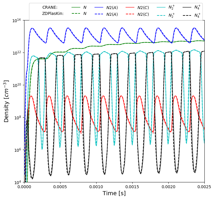
Nitrogen species and electrons versus time. Solid lines are computed by CRANE, dotted lines by ZDPlasKin.